






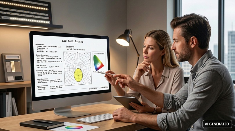
Every quality lighting project is born from information that is often overlooked: the photometric curve. It is a small, seemingly cryptic diagram that contains everything you need to know about how a light source will distribute its light in space. Knowing how to interpret the photometric curve means moving from buying by eye to designing methodically, predicting exactly where the light will fall, with what intensity and with what uniformity. In this in-depth guide we explain, step by step, what the photometric curve is, how to read it, what instruments generate it and, above all, why it is so important when working with LED strips.
Quick definition. The photometric curve is the graphical representation of the luminous intensity (measured in candelas) emitted by a source in every direction in space. Read on a polar diagram, it shows the shape of the light beam: how concentrated or diffuse it is, where it peaks and how it falls off at the sides. It is the fundamental tool for predicting the real illuminance of a fixture even before installing it.
Why the photometric curve matters more than ever today
We are experiencing an explosive growth in LED lighting. The global LED lighting market, valued at tens of billions of euros, is growing at double-digit rates, driven by energy efficiency, increasingly stringent regulations and the spread of flexible linear light sources. In this scenario, the ability to read a photometric curve is no longer a skill reserved for laboratory specialists, but a requirement for anyone who purchases, installs or designs lighting. LED strips, in particular, have made light a continuous architectural element, shifting the focus from mere lumen quantity to the distribution of that light: exactly what the photometric curve describes.
There is also an economic reason. A wrong lighting design is costly: fixtures that do not deliver the required lux have to be redone, incorrect optics create glare and shadow zones, overheated strips degrade prematurely. Learning to read the photometric curve before purchasing is the most cost-effective form of insurance against design errors. This is why we wrote this guide: to put a concrete tool in the hands of customers and designers to choose consciously among the hundreds of products in our catalog.
Photometric curve: the term in different languages
Those who work with international datasheets and software encounter the photometric curve under different names. In English it is referred to as photometric curve, light distribution curve or polar diagram; in Spanish as curva fotométrica or diagrama polar. The substance does not change: it is always the representation of luminous intensity as a function of angle. Recognizing these terms is useful because many IES and LDT files, as well as manuals from major manufacturers, are written in English. The classification of distributions (symmetrical, asymmetrical, batwing, Type I-V) also uses internationally shared terminology, which makes reading the photometric curve a transversal and universally applicable skill.
In this article...
1. What is photometry
Before being able to read a photometric curve you need to understand where it comes from. Photometry is the science that measures light as it is perceived by the human eye. Not all the energy emitted by a source is "light" in a useful sense: photometry deals exclusively with the portion of the electromagnetic spectrum that our visual system can see, weighting it to the actual sensitivity of the retina. It is the bridge between the pure physics of radiation and the concrete experience of a well-lit room.
Photometry originated as a branch of optical sciences and plays a central role in modern lighting design: without the measurement of light we could not compare two sources, design a system or certify the compliance of a fixture with regulations. Every LED strip we sell on Ledpoint.it is described through precise photometric quantities, and it is precisely photometry that provides the common language with which technicians, designers and installers communicate.
The definition of photometry
Photometry is the measurement of visible light in terms of its brightness as perceived by the human eye. Unlike a simple measurement of energy, it takes into account the fact that the eye is not equally sensitive to all wavelengths: it perceives green-yellow light (around 555 nanometers) as brighter than deep red or violet, even with the same emitted energy. This sensitivity is encoded in the so-called photopic sensitivity curve V(λ), the foundation of every photometric measurement.
Photometry and operating principle
The principle on which photometry is based is conceptually simple but technically sophisticated. An instrument called a photometer captures luminous radiation through a sensor (typically a photodiode) filtered to respond exactly like the human eye. The electrical signal produced is converted into a luminous quantity. Historically, before electronics, photometry was based on the visual comparison between two illuminated surfaces (a method linked to the Weber-Fechner law on the perception of stimuli) while today it relies on solid-state detectors calibrated with extreme precision.
Photometry is clearly distinguished from radiometry, which instead measures all radiant energy in watts without any perceptual filter. This difference is crucial: an infrared LED can emit a lot of radiant power but have a zero photometric value, because the eye cannot see it. We will explore this distinction further later, because it is the key to understanding why light is measured in lumens and not simply in watts.
What photometry is used for in lighting design
The applications of photometry are transversal. In lighting design it is used to size systems, in architecture to shape atmospheres, in photography to control exposure, in industry to guarantee quality control of the sources produced. For a technical e-commerce like Ledpoint, photometry is what allows us to honestly declare how many lumens an LED strip emits, with what efficiency (lumens/watt) and with what distribution: information that all flows into the product's photometric curve.
2. Photometric quantities: lumen, lux, candela
You cannot read a photometric curve without mastering the three fundamental quantities that describe light. They are often confused with each other, yet they represent completely different concepts: the total emitted flux, the intensity in a direction and the amount that reaches a surface. Clarifying this distinction is the first, indispensable step to correctly interpreting any photometric diagram.
The lumen: how much light the source emits
The lumen (lm) measures the luminous flux, i.e. the total amount of visible light emitted by a source in all directions. It is the data you find on the packaging of a light bulb or on the datasheet of an LED strip. A high-efficiency Ledpoint LED strip, for example, can reach 130 lm/W: this means that for every watt of electrical power absorbed it produces 130 lumens of light. The lumen, however, says nothing about where that light goes: and this is where the candela comes into play.
The candela: intensity in a direction
The candela (cd) measures luminous intensity, i.e. the flux emitted in a specific angular direction. It is the quantity that is actually plotted in the photometric curve: each point on the curve represents the value in candelas measured at a certain angle relative to the source's axis. A source with a narrow, concentrated beam will have many candelas forward and few at the sides; a diffuse source will distribute the candelas more uniformly. The candela, therefore, is the true protagonist of the polar diagram.
The lux: how much light reaches the surface
The lux (lx) measures illuminance, i.e. the amount of light that actually falls on a surface, equal to one lumen per square meter. It is the value we are interested in for the final result: how many lux are needed on a work plane, on a backlit shelf or on a step. The relationship between candela and lux goes through the inverse square law of distance: by doubling the distance from the source, the illuminance is reduced to a quarter. It is precisely the photometric curve, combined with distance, that allows you to calculate the expected lux at every point.
| Quantity | Symbol | Unit | What it describes | Role in the curve |
| Luminous flux | Φ | lumen (lm) | Total light emitted | Area of the photometric solid |
| Luminous intensity | I | candela (cd) | Light in a direction | Value plotted on the curve |
| Illuminance | E | lux (lx) | Light received by a surface | Result calculated from the curve |
| Luminance | L | cd/m² | Light perceived from a surface | Related to glare |
Mastering these four quantities (and in particular the difference between lux and lumen, between flux and intensity) is the basis for not being deceived by non-transparent product datasheets. Many manufacturers only declare total lumens, but it is the photometric curve that reveals how those lumens translate into real illuminance on the surface you care about.
3. What is the photometric curve
After defining photometry and its quantities, we can finally answer the central question: what exactly is a photometric curve? It is not a commercial datum or a graphic whim: it is the mathematical photograph of the luminous behavior of a fixture, obtained by measuring the intensity in candelas along all directions in space and plotting it on a diagram that can be read at a glance.
The precise definition of photometric curve
The photometric curve is the diagram that represents the distribution of the luminous intensity of a source as a function of the emission angle. In other words, it tells us how many candelas are emitted at 0°, 15°, 30°, 45° and so on, until covering the entire field around the source. What the photometric curve represents is therefore the "luminous signature" of the fixture: two LED strips with the same flux in lumens can have completely different curves, and therefore illuminate in a completely different way.
The term comes from the union of photometry (measurement of light) and the graphic form assumed by the data. In English it is called photometric curve or light distribution curve, in Spanish curva fotométrica: any international software or datasheet will use these terms, so it is useful to recognize them. On Wikipedia and in technical manuals you often find it associated with the concept of light distribution.
The polar diagram: the most common format
In the vast majority of cases the photometric curve is drawn on a polar diagram. Imagine the source at the center of a circle graduated in degrees: the perpendicular direction downward (for a ceiling light) or forward (for a spotlight) is 0°, while the sides extend towards ±90° and beyond. The concentric circles represent the intensity in candelas, like the contour lines of a map. The actual curve is the line that connects all the measured values: its shape immediately tells whether the beam is narrow, wide, symmetrical or asymmetrical.
Why represent light as a curve
We could list the intensity angle by angle in a table, and in fact digital files do this. But the human eye grasps a shape much more quickly than a column of numbers. The photometric curve compresses hundreds of measurements into a single image that can be interpreted in a few seconds: this is why it has become the universal standard in lighting catalogs. An experienced designer looks at the curve and already "sees" how the room will be lit, even before opening software.
On our product datasheets, the photometric curve of an LED strip or profile always accompanies the numerical data, because we believe that a professional customer should be able to evaluate not only how much light they are buying, but how that light will be distributed in their project.
Polar diagram and Cartesian diagram
In addition to the polar diagram, the photometric curve can also be represented in Cartesian form, with the angle on the horizontal axis and the intensity in candelas on the vertical axis. The Cartesian format is more precise for very narrow beams (such as those of spotlights) because it "stretches" the few central degrees across the entire width of the graph, where the polar diagram would compress them into a tiny space. In lighting practice, the polar diagram remains dominant for its visual immediacy, but knowing that the two formats describe the same data prevents confusion when moving from one catalog to another. Some manufacturers include both representations precisely to cover every reading need.
What the photometric curve does not say
It is also important to know what the photometric curve does not communicate. It does not describe the color of the light (temperature in kelvin), it does not indicate color rendering (CRI), it says nothing about any flicker nor about the build quality of the source. The photometric curve is a purely geometric map of the intensity distribution: fundamental, but always to be read together with the other parameters of the technical datasheet. Confusing the good shape of a curve with the overall quality of a product is a mistake that leads to incomplete choices.
4. How to read the photometric curve step by step
Many get stuck in front of that tangle of circles and numbers, but following an orderly method the reading becomes intuitive. Let's see together, step by step, how to read the photometric curve of any fixture, with particular attention to what matters for LED strips.
Step 1: identify the center and axes
The first gesture to read a photometric curve is to locate the center of the diagram, where the source is ideally located. From there starts the 0° axis, which represents the main direction of emission: downward for a ceiling light, forward for a spotlight. On both sides you find the angular graduations: +90° and −90° indicate horizontal emission, i.e. parallel to the installation surface. Recognizing these references is essential to avoid inverting the interpretation.
Step 2: read the scale in candelas
The concentric circles are the scale of luminous intensity, expressed in candelas. Attention: often the scale is normalized to 1000 lumens (cd/klm), so as to compare fixtures of different power. In this case, to obtain the real candelas, you multiply the value read by the actual lumens of your strip divided by one thousand. This detail is the source of one of the most frequent reading errors, as we will see later.
Step 3: follow the shape of the curve
The shape of the curve tells you everything about the light beam. If the line extends a lot along the 0° axis and narrows at the sides, the beam is concentrated (spot): it concentrates the light forward. If instead the curve is wide and flattened, with significant values even at 60-70°, the beam is wide (flood) and diffuses light over an extended area. Bare LED strips, typically, have a wide and rounded distribution, almost hemispherical, called Lambertian.
Step 4: identify the beam angle
The beam angle is conventionally defined as the opening within which the intensity is at least 50% of the peak value (half-intensity angle, FWHM). On the curve you identify it by finding the two angles, to the right and left, where the curve drops to half of its maximum. A profile with a narrow lens can take a strip from a wide 120° to a concentrated 30°, radically changing the result: and this is exactly what you read by comparing the two curves.
Step 5: evaluate symmetry and planes
Serious curves often show two superimposed lines: the longitudinal plane (C0-C180) and the transverse plane (C90-C270). For a linear LED strip these two planes are different, because the source is a segment and not a point: along the strip the light is continuous, while transversally it follows the Lambertian of the single chip. Reading both planes is essential to understand the real behavior of a linear source.
| Step | What to observe | What it reveals |
| 1 | Center and 0° axis | Main direction of light |
| 2 | Scale in candelas (or cd/klm) | Real or normalized intensity |
| 3 | Shape of the curve | Narrow or diffuse beam |
| 4 | Half-intensity angle | Beam angle (FWHM) |
| 5 | C0-C90 planes | Symmetry and linear behavior |
With these five steps you have a complete method to read any photometric curve. Practice will do the rest: after examining a dozen diagrams, you will recognize at a glance if a source is suitable for your project.
5. Types of photometric curve: symmetrical, batwing, type I-V
Not all photometric curves are the same. Indeed, recognizing which family a photometric curve belongs to is perhaps the most valuable skill, because each shape corresponds to an ideal application. In this section we classify the main types of light distribution, from the most common in LED strips to the standards used for street lighting.
Symmetrical photometric curve
A photometric curve is symmetrical when it distributes light identically around the vertical optical axis. This is the typical case of bare LED strips, panels and ceiling lights: the light radiates uniformly in all directions with the same pattern. Symmetry simplifies lighting calculation and guarantees homogeneous illumination, which is why it is the standard choice for general ambient lighting.
Batwing photometric curve ("bat wing")
The batwing photometric curve owes its name to the shape that resembles the spread wings of a bat: two pronounced lateral lobes and a central dip. This distribution deliberately reduces the intensity in the vertical direction to enhance it at the sides, thus obtaining extremely uniform illumination on wide surfaces without the annoying peak of light directly under the source. It is particularly appreciated in office lighting, corridors and linear ceiling lighting with LED strips and dedicated optics.
The Type I – Type V classes (IES standard)
In the North American IES standard, distributions for street and outdoor area lighting are classified into five types. Type I projects a narrow and long light, ideal for pedestrian paths; Type II and III progressively widen for roads and parking lots; Type IV projects forward for perimeter walls; Type V (Type V photometric curve) is circular and symmetrical, suitable for squares and intersections. Although it mainly concerns spotlights and street lamps, knowing this classification helps to interpret any international datasheet.
| Type of curve | Shape | Ideal application |
| Symmetrical (Lambertian) | Rounded hemispherical | Generic LED strips, panels, general lighting |
| Batwing | Two lateral lobes | Offices, corridors, uniform light lines |
| Concentrated (spot) | Narrow on the axis | Accent lighting, spotlights |
| Asymmetrical (wallwasher) | Shifted laterally | Wall washing, signs |
| Type I–V (IES) | From narrow to circular | Street and outdoor lighting |
6. From polar diagram to photometric solid
The photometric curve we see on paper is, in reality, a two-dimensional slice of a three-dimensional object. Understanding this passage greatly elevates the quality of reading, because light is not distributed on a plane but in space. Let us therefore introduce the concept of photometric solid and its link with the diagrams we have learned to read.
What is the photometric solid
The photometric solid is the three-dimensional surface obtained by representing the luminous intensity in every possible direction in space. If the photometric curve is a section, the photometric solid is the complete volume generated by rotating (or interpolating) all the sections around the source. The volume enclosed by this solid is proportional to the total luminous flux: this is why lumens correspond, geometrically, to the "area" of the photometric solid.
Why multiple measurement planes are needed
For a perfectly symmetrical source, a single photometric curve is enough to describe the entire solid, because it rotates identically on every plane. But for asymmetrical sources (and linear LED strips are) multiple sections are needed, typically the C0-C180 and C90-C270 planes. It is like describing a mountain: a single profile is not enough, you need multiple cuts to understand its real shape. The digital IES and LDT files store precisely this grid of planes.
Solar diagram, hypsometric curve and other relatives
It is worth clarifying a terminological point that generates confusion in searches. The solar diagram (or polar solar diagram) represents the path of the sun in the sky and is used for bioclimatic design, not for fixture photometry. The hypsometric curve, on the other hand, belongs to topography and describes the altitudes of a terrain. Although they share the polar or contour line shape with the photometric curve, they are tools of different disciplines: do not confuse them when searching for data on your fixtures.
7. The photometric curve of LED strips: why it is different
So far we have talked about photometry in general, but the real reason you opened this guide is probably only one: to understand the photometric curve of LED strips. LED strips have a peculiar luminous behavior, very different from that of a light bulb or a spotlight, and ignoring it leads to disappointing projects. Let's see why the LED photometric curve of a strip deserves special attention.
The linear source and Lambertian distribution
A single SMD LED chip emits light according to a Lambertian distribution: the maximum intensity is perpendicular to the surface of the chip and decreases with the cosine of the angle, reaching zero at 90°. This produces a typically rounded LED photometric curve, with an emission angle of about 120°. When many chips are aligned on an LED strip, the source becomes linear: along the axis of the strip the light is continuous and uniform, while transversally it preserves the Lambertian of the single emitter.
This is why the LED strip photometric curve almost always shows two distinct planes. If you search for the LED strip photometric curve of a product and only see one, it is probably the transversal section, the one that matters most to understand the beam opening. Our LED strips are accompanied by photometric data that describe both behaviors.
Why the photometric curve matters with LED strips
With an LED strip, the photometric curve tells you things that lumens alone could never reveal. It tells you, for example, whether the light will arrive uniformly at the bottom of a niche or whether it will create a central peak with shadowed edges. It tells you how visible the "dotted effect" of the individual chips will be. It tells you if a 120° strip is suitable for indirect ceiling lighting or if a narrower optic is needed. In a context where strips are used for backlighting, linear architectural lighting and accent lighting, this information is decisive.
COB vs SMD: two photometric curves compared
An emblematic case is the comparison between traditional SMD strips and COB (Chip On Board) strips. Our Ledpoint COB strips distribute the chips under a continuous phosphor coating, eliminating the dotted effect and producing a homogeneous line of light with a wide diffusion angle. On the photometric curve, this translates into a more regular distribution free of the small ripples typical of individual SMDs. If visual uniformity is the priority of your project, the COB curve speaks for itself.
Photometric curve of LED tube, reflector and panel
The reasoning about strips extends to other formats. The LED tube photometric curve resembles that of a coated strip, with linear 120° distribution; the LED reflector photometric curve is instead concentrated, because the reflector redirects the light forward; the LED panel photometric curve is wide and diffuse, ideal for uniform ceiling lighting. In each case, the reading method remains the same: only the shape the graph assumes changes.
LED photometric curve and comparison with traditional sources
It is worth comparing the LED photometric curve with that of the sources that LEDs have replaced. A fluorescent lamp, for example, emits light at 360° around the tube, with a photometric curve that is substantially circular and requires reflectors to be directed; a halogen lamp instead concentrates the light forward through its reflector. The LED, being intrinsically directional (it only emits from the chip side), starts with a huge efficiency advantage: it does not waste light backwards. This is one of the reasons why the photometric curve of an LED source is almost always more "useful" (the light goes where it is needed) than that of previous technologies such as fluorescent, halogen or discharge lamps.
Chip density and curve fineness
A final aspect specific to strips: the overall photometric curve of the light line also depends on the density of the chips. At low density, between one LED and the other the intensity drops, creating micro-oscillations in the longitudinal distribution that translate into the visible "dotted effect". At high density or with COB technology, these oscillations disappear and the longitudinal photometric curve becomes a continuous and regular line. This is why, for applications where the strip is visible or reflects on glossy surfaces, the density of the LEDs must be evaluated with the same attention dedicated to the transversal shape of the curve.
8. How profiles and diffusers modify the photometric curve
Here is an aspect that few consider and which is instead among the most important of all: the photometric curve of an LED strip is not fixed. It changes (and even radically) depending on the aluminum profile and the diffuser in which you install it. Ignoring this means designing on the wrong curve. Let's see how Ledpoint accessories transform the light distribution.
The role of the diffuser
A bare LED strip is, in fact, a row of very intense luminous dots: looking at it directly is annoying and dazzling (discomfort glare). The diffuser mounted on the profile transforms those dots into a continuous and uniform line of light, but in doing so it modifies the photometric curve. Not all diffusers are the same, and the choice directly affects efficiency and beam shape.
| Diffuser | Efficiency loss | Effect on the curve | Ideal use |
| Transparent (clear) | Minimal | Curve almost unchanged, LEDs visible | Maximum light output |
| Opal (opal) | ~10-15% | Wider and softer curve, reduced peak | Best compromise, uniformity |
| Microprismatic | Variable | Control of the emission angle | Accent lighting |
Profiles and beam direction
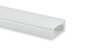
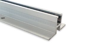
The geometry of the profile also determines the direction in which the light is emitted. Profiles can orient the beam downward (direct lighting), upward (indirect), laterally or in bi-emission. An angular profile mounted in a perimeter niche, for example, produces an asymmetrical photometric curve that "washes" the adjacent wall. Choosing the right profile literally means choosing the right curve. Explore our range of aluminum profiles for LED strips to understand how many configurations are possible.
Thermal dissipation and curve stability over time
An aspect often overlooked: the declared photometric curve is only valid if the LED works at the correct temperature. An overheated strip reduces the flux and degrades faster. Aluminum profiles, with their excellent thermal conductivity (about 235 W/m·K), act as passive heatsinks keeping the LEDs at the optimal operating temperature. They not only improve the shape of the curve thanks to the diffuser, but ensure that that curve remains stable for all the declared 30,000 hours. Explore the topic further with our guide on what aluminum profiles for LEDs are for.
9. The tools: goniophotometer, lux meter, IES and LDT files
A reliable photometric curve is not improvised: it is born from measurements performed with precision instruments in certified laboratories. Knowing these tools helps you evaluate the seriousness of a datasheet and understand what checks you can do yourself in the field. This section answers the questions of those who, like the engineer or researcher, want to understand the "how" of the measurement.
The goniophotometer
The goniophotometer is the instrument that generates the photometric curve. It consists of a mechanical system that rotates the source (or a mirror, or the sensor) around two axes, measuring the luminous intensity at every angle with a calibrated photometer. The result is the complete grid of values in candelas from which the curves and the photometric solid are built. There are rotating mirror goniophotometers, moving arm goniophotometers and rotating source goniophotometers, each with specific advantages for the type of fixture.
The photometer and the lux meter
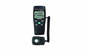
The photometer measures luminous quantities as they are perceived by the human eye, thanks to a sensor filtered on the V(λ) curve. The lux meter is a photometer calibrated to measure illuminance in lux on a surface: it is the most widespread instrument for field checks, the one that a lighting designer like Sara would use to verify that a work plane actually receives the design lux. It is inexpensive, portable and indispensable to validate that reality reflects the starting photometric curve.
The integrating sphere
To measure the total luminous flux in lumens, the integrating sphere (Ulbricht sphere) is used: a spherical cavity with a highly reflective internal coating in which the source is placed at the center. The light is integrated over the entire internal surface and is read by a single sensor, returning the total flux regardless of direction. It is complementary to the goniophotometer: the sphere says how much, the goniophotometer says where.
IES and LDT files: the curve in digital format
In the era of computer-aided design, the photometric curve travels in digital format. The two standards are the IES file (.ies extension, North American IESNA LM-63 standard) and the LDT file (EULUMDAT, widespread in Europe). Both contain the complete matrix of luminous intensities for every plane and angle, in addition to flux and power data. They are structured text files that any lighting software can import to reconstruct curves, photometric solid and simulations. When you download an IES file from a product datasheet, you are downloading the complete and usable photometric curve of your fixture.
10. Using the photometric curve in DIALux and Relux
Knowing how to read the photometric curve is the first step, while the second is to put it to work in a real project. This is where lighting calculation software comes into play, transforming photometric files into photorealistic simulations and regulatory compliance reports. Let's see how the photometric curve integrates in DIALux, the most widespread tool in the sector.
Importing the photometric file
The workflow starts with importing the IES or LDT file into the software. DIALux and Relux read the DIALux photometric curve of the product and associate it with a 3D model of the fixture. From that moment on, the software knows exactly how that source distributes light and can calculate the illuminance on any surface of the scene. For LED strips it is possible to define continuous light lines by applying the curve of the single module per linear meter.
The simulation: from candelas to lux on the scene
Once the fixtures are positioned, the software applies the inverse square law and the geometry of the room to calculate the lux at every point. The result is a lighting verification: isolux maps, average and minimum values, uniformity, UGR glare index. All this derives directly from the starting photometric curve. If the curve is inaccurate, the entire simulation will be: this is why demanding serious photometric data from the supplier is fundamental.
Reading a lighting verification
The final report is the document that the designer delivers to the client and, often, the one that demonstrates compliance with regulations such as UNI EN 12464-1 (lighting of indoor workplaces). Reading a lighting verification means checking that the maintained average illuminance respects the regulatory minimums, that the uniformity is adequate and that the glare is below threshold. Every single number in that report has its root in the photometric curve of the chosen fixtures.
11. Real use cases with Ledpoint LED strips
Theory comes to life when it is applied. In this section we translate the photometric curve into concrete design decisions, showing how the correct reading of the light distribution guides the choice of the LED strip, profile and diffuser in real scenarios. These are the same reasonings that our customers (designers, installers, designers) face every day.
Indirect ceiling lighting (cove lighting)
For indirect lighting that washes the ceiling uniformly, a wide and soft photometric curve is needed, free of concentrated peaks. The ideal choice is a high-density LED strip mounted in a perimeter profile with an opal diffuser: the resulting curve, wide and flattened, avoids streaks on the ceiling. In these applications, with high CRI LED strips (≥ 90-95) and warm temperature 2700-3000K, the diffused light enhances the surfaces without dazzling. Our high-efficiency LED strip lines, up to 130 lm/W, are designed exactly for this.
Backlighting and glass shelves
To backlight a piece of furniture, a shelf or a ledge, the LED strip photometric curve must be as uniform as possible to avoid visible "hot spots" through the glass. Here the COB strip is unbeatable: its regular curve free of dotting creates a continuous blade of light. Combined with a small profile, it allows elegant integrations. Discover our solutions for LED backlighting.
Linear architectural lighting on curves and corners
When the project requires following curved surfaces, the geometry of the source matters as much as the light curve. The Ledpoint Zig-Zag foldable LED strips can bend not only along the longitudinal axis but also horizontally and in curves, maintaining a coherent photometric curve even on corners. This avoids light interruptions and intensity variations that ruin a continuous light line.
Directional accent lighting
To illuminate a painting, an object in a showcase or an architectural detail, a concentrated photometric curve is needed. In this case a profile with a microprismatic diffuser or with dedicated optics is chosen, which narrows the emission angle from the typical 120° to much narrower values. The curve extends along the axis and the beam becomes directional, highlighting the subject without dispersing light into the environment.
| Application | Ideal curve | Recommended Ledpoint product |
| Indirect ceiling lighting | Wide and soft | High density strip + opal profile |
| Furniture backlighting | Uniform, no hot spots | COB strip |
| Curves and corners | Coherent on corners | Zig-Zag foldable strip |
| Accent lighting | Concentrated | Microprismatic profile / narrow optics |
| Waterproof outdoor | Diffuse, IP protection | IP65/IP68 strip |
12. Common mistakes when reading the photometric curve
Even expert technicians fall into recurring traps when interpreting a photometric curve. Recognizing them in advance saves you wrong projects and disappointments on site. Here are the mistakes we see most often and how to avoid them.
Mistake 1: confusing lumens and candelas
Reading the value on the curve as if they were lumens is the number one mistake. The curve reports candelas (intensity in a direction), not the total flux in lumens. Two strips with the same flux can have very different candela peaks depending on how much they concentrate the light. Always remember: lumens are the volume of the solid, candelas are its extension in a direction.
Mistake 2: ignoring the 1000 lm normalization
Many curves are normalized in cd/klm to make different fixtures comparable. If you forget to rescale to the real flux of your strip, you will get completely wrong illuminance values. Always check if the scale is in absolute or normalized candelas.
Mistake 3: reading only one plane of a linear source
With LED strips, evaluating only the transversal plane and ignoring the longitudinal one leads to underestimating the uniformity along the strip or overestimating the concentration. Linear sources require reading both planes.
Mistake 4: forgetting the effect of the diffuser
The photometric curve of the bare strip is not the one you will have once you install the profile with the diffuser. As seen, the opal widens and attenuates, the microprismatic concentrates. Always design on the curve of the complete system, not just the LED.
Mistake 5: neglecting the operating temperature
The declared curve is valid at a precise junction temperature. If the strip works overheated because it lacks dissipation, the real flux will be lower and the curve will "drop". A good aluminum profile is what keeps the curve faithful over time.
13. Physical principles and history of photometry
To fully appreciate the meaning of a photometric curve it is advisable to take a step back and understand where our ability to measure light comes from. Photometry has its roots in centuries of studies on visual perception and the physics of radiation, and the way we draw a photometric curve today is the direct heir of those insights. Knowing its principles is not an academic exercise: it is what allows you to correctly interpret every number you will find on a datasheet.
From the historical candle to the modern candela
The term "candela" is not random. Originally, luminous intensity was measured against the light emitted by a standardized spermaceti candle: hence the unit "candlepower". The modern definition is much more rigorous and links the candela to a precise amount of radiation at 540 terahertz, but the underlying concept remains the same: to quantify how much light travels in a specific direction. Every point of a photometric curve is, essentially, a value heir to that ancient reference candle.
The Weber-Fechner law and perception
A conceptual pillar of photometry is the Weber-Fechner law, according to which the perception of a stimulus grows logarithmically with respect to the physical intensity of the stimulus itself. In practice, the human eye does not perceive light in a linear way: doubling the lumens does not double the sensation of brightness. This principle explains why photometry must weight measurements on the real response of the eye and not on pure physical energy, and why the perception of uniformity of a photometric curve does not mechanically coincide with its numerical values.
The light spectrum and the V(λ) curve
Visible light occupies a narrow band of the electromagnetic spectrum, between about 380 and 780 nanometers. Within this band, the eye reaches maximum sensitivity around 555 nm (green-yellow) in daylight vision. The curve that describes this sensitivity, the luminous efficiency function V(λ), is the heart of every photometric measurement: it is the filter that converts radiometric energy into photometric quantities. When a laboratory builds a photometric curve, its sensors must faithfully replicate this sensitivity curve, otherwise the data would be falsified.
For LED strips this aspect is particularly relevant: two strips with the same spectrum but different spectral distribution can produce the same value in lumens but a very different light quality (CRI, color temperature). The photometric curve describes the spatial distribution of light, while the spectrum describes its chromatic quality: two complementary pieces of information that together completely define a source.
14. Applications of photometry and the photometric curve
Photometry and the photometric curve do not belong to a single sector: they are transversal tools that cross engineering, architecture, photography, industry and research. Let's see the main fields of application, because understanding "what it is for" helps to give meaning to every technical datum.
Lighting design and architecture
It is the natural realm of the photometric curve. Every lighting project (an office, a museum, a facade, a shop) starts with the choice of fixtures with the appropriate light distribution. The architect and the lighting designer use the photometric curve to model light as a design material: deciding where to concentrate it, where to diffuse it, how to avoid glare and unwanted shadows. With LED strips, this means composing light lines that follow the architecture without ever betraying it.
Photography and cinematography
In the world of image, photometry controls exposure and light quality. A professional photographer measures illuminance and color temperature to obtain consistent and repeatable results. High CRI LED strips are increasingly used as continuous light in the studio precisely because they offer faithful color rendering and, thanks to the known photometric curve, predictable distribution on the subject.
Industry and quality control
In the production of light sources, photometry is the quality control tool par excellence. Every batch of LEDs is checked for flux, efficiency, color temperature and distribution. This is why serious strips, such as those built with 3-step MacAdam chip selection, guarantee chromatic coherence between different batches: without photometric measurement there would be no way to ensure it.
Public and street lighting
For those who manage public lighting systems, the photometric curve is at the center of regulatory compliance. Type I-V classes, uniformity on the road surface, light pollution control and energy efficiency all depend on the correct choice of light distribution. A well-designed photometric curve reduces consumption by illuminating only where needed, while improving night safety.
15. Calibration and accuracy of photometric measurements
A photometric curve is worth as much as the instrumentation that produced it. For this reason calibration and accuracy control are technical aspects that separate a serious datum from an invented one. This section answers the needs of those who, like the engineer Marco or the researcher Luca, must trust the numbers or even produce them.
How photometric instruments are calibrated
Photometric instruments are calibrated by comparing them with reference sources traceable to national and international standards. A lux meter, for example, is calibrated on a reference source of known illuminance; a goniophotometer is verified with reference lamps of certified intensity. Periodic calibration is essential because sensors and optical components drift over time, and a photometric curve measured with uncalibrated instruments would be systematically wrong.
Sources of error to control
The accuracy of a photometric curve depends on the control of numerous variables: the correct spectral response of the sensor (f1' error), the cosine angular response for lux meters (f2' error), the thermal stabilization of the source during the measurement, the absence of stray light in the laboratory. LED strips, in particular, require a stabilization period before the measurement, because the flux varies while the LED reaches the steady-state temperature. Neglecting these precautions produces optimistic curves that then do not find confirmation in the field.
Why to trust (or distrust) a datasheet
A serious datasheet declares the measurement conditions: ambient temperature, driving current, stabilization time. When this data is missing, the provided photometric curve should be taken with caution. At Ledpoint we make photometric files available so that every designer can independently verify the expected behavior.
16. Professionals' questions about the photometric curve
Every professional figure looks at the photometric curve with different eyes. We have collected the most typical questions of those who work with light every day and we answer them in a targeted way, because the needs of an engineer are not those of a photographer or a lighting designer.
The engineer: reliability and integration
Those who design systems wonder which photometric instruments are most reliable for precision measurements and how to integrate data into their automation flows. The answer lies in the measurement chain: accredited goniophotometer for the photometric curve, integrating sphere for flux, and IES/LDT files as the standard exchange format towards software. Correctly interpreting photometric data means always tracing back to the measurement conditions and not taking peak values as absolute guarantees. Integration happens through photometric files, today the universal standard importable in every calculation environment.
The researcher: materials and controlled environments
Those who analyze optical materials in the laboratory need controlled environments, stable sources and low-uncertainty sensors. The main challenges concern repeatability and the separation between photometric and radiometric quantities when studying materials that also respond outside the visible spectrum. For these applications, the photometric curve is often accompanied by complete spectral measurements, because spatial distribution alone is not enough to characterize a material.
The lighting designer: evaluating the effect in space
The designer wants to evaluate the effect of lighting in a real space and measure the distribution of light in complex environments. Here the photometric curve is the starting point for the DIALux simulation, while the lux meter serves for the final field verification. The best way to calibrate the lights in a design project is to compare the measured lux with the simulated ones, correcting position and optics until the result coincides with the design intent. LED strips offer unique flexibility here, allowing you to model linear light point by point.
The plant manager: efficiency and regulations
Those who manage public lighting focus on energy efficiency, regulatory compliance and maintenance. The photometric curve guides the choice of fixtures that illuminate the road surface uniformly, reducing the number of light fixtures and consumption. Interpreting photometric data in this context means reading isolux curves and verifying the uniformity required by regulations, guaranteeing night safety without waste.
The photographer: color temperature and rendering
The photographer wonders how to measure the color temperature of lights and interpret the data to improve shots. Here, in addition to the photometric curve that describes the distribution, CRI and correlated color temperature (CCT) come into play. High CRI LED strips (≥ 95) with controlled CCT are the ideal choice for faithful continuous light, and their known photometric curve allows you to predict how the light will fall on the subject even before turning it on.
17. Technical parameters of LED strips beyond the photometric curve
The photometric curve does not live in isolation: it intertwines with other technical parameters that, together, define the quality of an LED strip. Knowing them all allows you to read a product datasheet in its entirety and choose wisely.
LED density and uniformity
The number of LEDs per meter directly affects uniformity and, indirectly, the perceived photometric curve. A low-density strip shows distinct dots; a high-density or COB strip produces a continuous line. Our strips declare the cutting pitch (for example every 3, 6 or 8 LEDs) which indicates both the installation flexibility and the fineness of the obtainable light line.
Color temperature and CRI
The color temperature, expressed in kelvin, ranges from warm white (2200-3500K) to cold white (5500-8700K) up to ice white. The CRI (color rendering index) measures how faithfully colors appear under that light. For accent and retail lighting, high CRIs are preferred, while the photometric curve decides where that quality light will fall. Ledpoint offers strips divided precisely by color temperature, from warm to ice, in addition to RGB, RGBW and adjustable CCT.
IP protection rating
For outdoor applications or in humid environments, the IP protection rating (from IP20 to IP68) determines resistance to dust and water. Our IP65 and IP68 strips are designed for outdoors, swimming pools and harsh environments. Attention: the protection, by encapsulating the strip, can slightly modify the photometric curve and reduce the output flux, a datum we always declare honestly.
Power, efficiency and power supply
The power per meter (from 4.8 to over 14.4 W/m) and the efficiency in lumens/watt determine how much light you get and at what energy cost. The strips must be paired with adequate power supplies (5V, 12V, 24V, 48V) and, if necessary, with anti-flicker drivers. The correct choice of power supply ensures that the strip works at the point where the declared photometric curve is valid, without flux drops or flicker.
| Parameter | Typical Ledpoint range | Impact on the project |
| Efficiency | up to 130 lm/W | Consumption and light output |
| Color temperature | 2200-15000K | Atmosphere and visual comfort |
| CRI | up to ≥95 | Color fidelity |
| IP protection | IP20 – IP68 | Indoor/outdoor use |
| Power | 4.8 – 14.4+ W/m | Light intensity |
| Lifespan | ~50,000 hours | Curve stability over time |
Reading the photometric curve together with these parameters gives you the complete picture: you know how much light, of what quality and where it will end up. It is the approach we recommend to anyone who wants to design with LED strips as a professional would.
18. How to calculate lux starting from the photometric curve
One of the moments when the photometric curve stops being theory and becomes a project is the calculation of illuminance. Knowing how many candelas a source emits in a direction allows you to predict how many lux will arrive on a surface at a certain distance. Let's see the method, simplified but correct, which is the basis of every lighting verification.
The inverse square law
The fundamental principle is the inverse square law of distance: the illuminance (in lux) on a surface perpendicular to the light ray is equal to the luminous intensity (in candelas read on the photometric curve) divided by the square of the distance in meters. In formula: E = I / d². If a source emits 1000 candelas in a direction and the surface is 2 meters away, the illuminance will be 1000 / 4 = 250 lux. By doubling the distance to 4 meters, the lux drops to 1000 / 16 = 62.5 lux. This is why distance is so critical in projects.
The correction of the angle of incidence
The previous formula is valid if the light hits the surface perpendicularly. When instead it arrives at an angle, Lambert's cosine law comes into play: the real illuminance is obtained by multiplying by the cosine of the angle of incidence. A light that hits at 60° from the perpendicular provides only half of the illuminance (cosine of 60° = 0.5). For this reason, in projects with lateral or inclined LED strips, reading the photometric curve and correcting for the angle is essential to avoid overestimating the useful light.
A practical example with an LED strip
Imagine an LED strip mounted on the ceiling to illuminate a work plane at 2.5 meters. From the photometric curve you read the downward intensity, let's say 400 cd per linear meter (on a real scale). The direct illuminance under the strip will be about 400 / 2.5² = 64 lux per meter of strip. Adding the contribution of multiple meters and the reflections from the walls — which the software calculates automatically — you obtain the average illuminance of the scene. This simple example shows how the photometric curve is the direct bridge between the technical datum and the real lux on the work plane.
When software is needed and when manual calculation is enough
Manual calculation is useful for quick estimates and to understand orders of magnitude, but it neglects surface reflections, shading and the overlap of multiple sources. For a professional project that must comply with UNI EN 12464-1, software with photometric files remains irreplaceable. However, knowing how to do the calculation by hand (even just to verify that the software result is plausible) is a skill that distinguishes the true technician. And everything starts, once again, from the correct reading of the photometric curve.
19. Basic photometric glossary
To fix the concepts, here is a glossary of the terms you encounter most often working with the photometric curve and with LED strips. Keep it handy when you read a technical datasheet: many misunderstandings arise simply from definitions taken for granted.
| Term | Definition |
| Luminous flux | Total amount of visible light emitted, in lumens (lm). |
| Luminous intensity | Light emitted in a direction, in candelas (cd); it is what the photometric curve plots. |
| Illuminance | Light that arrives on a surface, in lux (lx = lm/m²). |
| Luminance | Light emitted or reflected by a surface towards the eye, in cd/m²; related to glare. |
| Luminous efficiency | Lumen/watt ratio: how much light is obtained per unit of power. |
| CRI | Color rendering index: fidelity with which colors appear under the light (max 100). |
| CCT / Kelvin | Correlated color temperature: warm (low K) or cold (high K). |
| Beam angle | Opening within which the intensity is ≥ 50% of the peak (FWHM). |
| Lambertian | Distribution in which the intensity decreases with the cosine of the angle; typical of bare LEDs. |
| Photometric solid | 3D surface of the luminous intensity in all directions. |
| IES / LDT files | Digital formats of the photometric curve for calculation software. |
| Goniophotometer | Instrument that measures intensity at every angle to build the photometric curve. |
| UGR | Unified Glare Rating: glare evaluation index. |
| IP rating | Protection against dust and water (e.g. IP65, IP68). |
With this vocabulary you master the language with which the photometric curve and its surrounding data are described in any catalog or professional software. Every term is a piece that, united with the others, allows you to read a lighting project with the confidence of an expert.
19. Photometry and radiometry: the distinction that explains everything
Before closing, it is worth returning to a distinction that is at the root of every photometric curve and that answers a recurring question among engineers and researchers: why is light measured in lumens and not simply in watts? The answer separates two sister but different disciplines.
Radiometry measures all radiant energy, in watts, without any reference to the human eye. An infrared emitter, invisible to us, has high radiometric values. Photometry, on the other hand, measures only the visible portion, weighted on the sensitivity of the retina through the V(λ) curve. It is this "perceptual filter" that transforms radiometric watts into photometric lumens. This is why two sources with the same electrical power can have very different luminous fluxes: the conversion efficiency and the emitted wavelength matter.
This is why the efficiency of an LED strip is expressed in lumens/watt and not in a simple percentage: it relates the photometric quantity (lumens) with the electrical one (watts). And for this reason the photometric curve — built in candelas, a photometric quantity — describes the useful and perceivable light, the only one that counts when you design an environment for real people.
| Aspect | Radiometry | Photometry |
| What it measures | All radiant energy | Only perceived visible light |
| Reference to the eye | None | Photopic V(λ) curve |
| Flux unit | Watt (W) | Lumen (lm) |
| Intensity unit | W/sr | Candela (cd) |
| Typical application | Physics, sensors, IR/UV | Lighting design, design |
20. Frequently asked questions about the photometric curve
We collect here the most frequent questions we receive about photometry, photometric curve and LED strips, with concise and direct answers. Click on each question to open the answer.
What is the photometric curve?It is the graphical representation of how a source distributes its luminous intensity (in candelas) in space. It describes how much light is emitted in each angular direction, allowing you to predict the illuminance and performance of a fixture before installation. |
How do you read the photometric curve?You start from the center of the polar diagram, where 0° is the direction perpendicular to the source. The concentric circles indicate the intensity in candelas: the more the curve extends in a direction, the more light is emitted there. The shape reveals if the beam is concentrated or diffuse. |
What is the photometric curve of LED strips used for?It is used to predict how an LED strip will illuminate a surface, choose the right profile and diffuser, calculate the illuminance in lux and avoid shadow areas or glare. It transforms technical specifications into a reliable lighting design. |
What is the difference between symmetrical and batwing curve?The symmetrical curve distributes light equally around the axis, typical of bare Lambertian strips. The batwing ("bat wing") concentrates light laterally and reduces vertical intensity: ideal for illuminating wide surfaces uniformly, without a central peak. |
What are IES and LDT files?They are the digital formats of the photometric curve: IES is the North American standard (IESNA), LDT the European format (EULUMDAT). They contain the complete matrix of luminous intensities and are imported into software such as DIALux or Relux to simulate real lighting. |
What is the difference between photometry and radiometry?Radiometry measures all radiant energy in watts, without filters. Photometry measures only visible light, weighted on the sensitivity of the eye (V-lambda curve). This is why lumens, lux and candelas are used instead of watts. |
What instruments are needed to measure the photometric curve?The goniophotometer generates the curve by rotating the source or sensor to detect intensity at every angle. The lux meter measures lux in the field, the integrating sphere the total flux in lumens. A photometer measures the quantities perceived by the human eye. |
How does the photometric curve change with the aluminum profile?The profile and its diffuser modify the curve: the opal widens and softens the beam reducing the peak (~10-15%), while a microprismatic or a narrow lens concentrates the light by narrowing the emission angle for more directional accent lighting. |
21. From theory to practice: choosing and installing the right strip
All the theory on light distribution serves only one purpose: to make better choices on site. In this section we translate everything into a concrete decision-making path, from design to installation, so as to put to use what you have learned by reading this guide. It is the final bridge between the graph on paper and the light you will see turn on in the room.
Defining the lighting objective
The first step is not technical but design-related: what do you want to achieve? A diffuse general lighting, an accent on a detail, a decorative line, a soft backlighting? Each objective requires a different light distribution and, consequently, a different combination of strip, profile and diffuser. Clearly defining the intent avoids choosing oversized or inadequate products. A work environment requires uniformity and visual comfort; a showcase requires contrast and directionality; a living room requires warmth and atmosphere.
Choosing color temperature and CRI
Once the objective is defined, the quality of light is chosen. For domestic environments and hospitality, warm white (2700-3000K) is preferred, which creates intimacy; for offices and kitchens, natural white (4000K); for specific technical and commercial applications, cold white. The CRI is chosen according to the importance of colors: high for retail, art and photography, standard for functional applications. Ledpoint offers a complete range of temperatures, from warm white 2200K to ice white over 9000K, in addition to adjustable CCT solutions that allow you to vary the tone at will.
Sizing power and power supply
The power per meter determines the luminous intensity: low values (4.8 W/m) for decorative accents, high values (14.4 W/m and over) for main lighting. The correct power supply must then be chosen for voltage (12V, 24V, 48V) and power, with a safety margin of about 20% compared to the load. For long runs, voltage drop must be evaluated, powering the strip from both ends or using constant current strips that maintain constant brightness over the entire length. Correct sizing is what ensures that the source works at the point where its declared data are valid.
Selecting profile and diffuser
Here everything we have said about light distribution comes back into play: the profile determines direction and dissipation, the diffuser determines uniformity and beam opening. For a continuous light line free of dots, a profile with an opal diffuser is chosen; for accent, a microprismatic one; for maximum output, a transparent one. The choice of the right profile is, as we have seen, the choice of the right curve. Ledpoint offers recessed, surface-mounted, angular, walkable, suspended, waterproof and decorative profiles, each with dedicated diffusers.
Installing correctly to preserve performance
Installation affects the final performance. The double-sided tape adheres well only on clean, unpainted surfaces, at a temperature between 21 and 38°C, and reaches full hold after about 72 hours. The strip must always be housed in the aluminum profile to dissipate heat: sticking it directly on wood or plasterboard drastically reduces its useful life. Cuts must only be made on the indicated points, soldering or connectors must be performed to the highest standard, and for outdoors the declared IP rating must be respected. Taking care of the installation means ensuring that the real light corresponds to the designed one.
| Step | Decision | Guiding question |
| 1 | Objective | What effect do I want to achieve? |
| 2 | Light quality | Which color temperature and CRI? |
| 3 | Power | How many W/m and which power supply? |
| 4 | Optics | Which profile and diffuser? |
| 5 | Installation | How do I preserve dissipation and IP? |
By following this path and knowing how to interpret light distribution data, anyone can move from improvised purchases to solid and repeatable projects. It is exactly the level of competence we want to transfer to our customers, because a customer who chooses well is a customer satisfied with the result.
22. Photometric curve: a tool serving designers
Knowing how to read a photometric curve is what distinguishes those who buy light from those who design it. We have seen that the photometric curve is not a technical detail reserved for specialists, but the most direct tool to predict the real behavior of a source: from photometry as the science of perceived light, to the quantities of lumen, candela and lux, up to the practical reading of the polar diagram and the use in software such as DIALux.
With LED strips, in particular, the photometric curve becomes decisive: the linear nature of the source, the effect of the diffuser, the choice of the profile and the thermal dissipation modify its shape and, with it, the final result of your project. Mastering this reading allows you to consciously choose between a uniform COB strip, a foldable one for corners or a concentrated optic for accent.
On Ledpoint.it you find LED strips, aluminum profiles, diffusers and professional power supplies, accompanied by the photometric data necessary to design without surprises. If you have a specific project, our technical team is available to help you choose the right LED strip for every application.
This article was developed with the support of artificial intelligence and subsequently reviewed, corrected, and validated by the Ledpoint.it technical team, which guarantees its reliability and compliance with official sources.